머신러닝
Kaggle-Titanic-predicted sirvived
easysheep
2023. 3. 30. 17:35
1. 문제 출처 및 참고한 사람
문제: https://www.kaggle.com/competitions/titanic
Titanic - Machine Learning from Disaster | Kaggle
www.kaggle.com
참고:https://www.kaggle.com/code/omarelgabry/a-journey-through-titanic/notebook
A Journey through Titanic
Explore and run machine learning code with Kaggle Notebooks | Using data from Titanic - Machine Learning from Disaster
www.kaggle.com
2. 문제 풀이
# 필요한 라이브러리 불러오기

# 데이터 분석
import pandas as pd
import numpy as np

# 데이터 시각화
import matplotlib.pyplot as plt
import seaborn as sns
# 눈금 그리기
sns.set_style('whitegrid')
%matplotlib inline

# 머신러닝 모델 불러오기

## 로지스틱 회귀
from sklearn.linear_model import LogisticRegression
## SVC  서포터 백터 머신
from sklearn.svm import SVC
## 랜덤 포레스트
from sklearn.ensemble import RandomForestClassifier

## for validation data
from sklearn.model_selection import train_test_split
In [114]:
# 데이터 불러오기
train_df = pd.read_csv("./titanic/train.csv")
test_df = pd.read_csv("./titanic/test.csv")
In [115]:
train_df.head(10)
Out[115]:
PassengerIdSurvivedPclassNameSexAgeSibSpParchTicketFareCabinEmbarked0123456789
| 1 | 0 | 3 | Braund, Mr. Owen Harris | male | 22.0 | 1 | 0 | A/5 21171 | 7.2500 | NaN | S |
| 2 | 1 | 1 | Cumings, Mrs. John Bradley (Florence Briggs Th... | female | 38.0 | 1 | 0 | PC 17599 | 71.2833 | C85 | C |
| 3 | 1 | 3 | Heikkinen, Miss. Laina | female | 26.0 | 0 | 0 | STON/O2. 3101282 | 7.9250 | NaN | S |
| 4 | 1 | 1 | Futrelle, Mrs. Jacques Heath (Lily May Peel) | female | 35.0 | 1 | 0 | 113803 | 53.1000 | C123 | S |
| 5 | 0 | 3 | Allen, Mr. William Henry | male | 35.0 | 0 | 0 | 373450 | 8.0500 | NaN | S |
| 6 | 0 | 3 | Moran, Mr. James | male | NaN | 0 | 0 | 330877 | 8.4583 | NaN | Q |
| 7 | 0 | 1 | McCarthy, Mr. Timothy J | male | 54.0 | 0 | 0 | 17463 | 51.8625 | E46 | S |
| 8 | 0 | 3 | Palsson, Master. Gosta Leonard | male | 2.0 | 3 | 1 | 349909 | 21.0750 | NaN | S |
| 9 | 1 | 3 | Johnson, Mrs. Oscar W (Elisabeth Vilhelmina Berg) | female | 27.0 | 0 | 2 | 347742 | 11.1333 | NaN | S |
| 10 | 1 | 2 | Nasser, Mrs. Nicholas (Adele Achem) | female | 14.0 | 1 | 0 | 237736 | 30.0708 | NaN | C |
In [116]:
# 데이터의 전체적인 정보 확인
train_df.info()
print("="*60)
test_df.info()
<class 'pandas.core.frame.DataFrame'>
RangeIndex: 891 entries, 0 to 890
Data columns (total 12 columns):
 #   Column       Non-Null Count  Dtype
---  ------       --------------  -----
 0   PassengerId  891 non-null    int64
 1   Survived     891 non-null    int64
 2   Pclass       891 non-null    int64
 3   Name         891 non-null    object
 4   Sex          891 non-null    object
 5   Age          714 non-null    float64
 6   SibSp        891 non-null    int64
 7   Parch        891 non-null    int64
 8   Ticket       891 non-null    object
 9   Fare         891 non-null    float64
 10  Cabin        204 non-null    object
 11  Embarked     889 non-null    object
dtypes: float64(2), int64(5), object(5)
memory usage: 83.7+ KB
============================================================
<class 'pandas.core.frame.DataFrame'>
RangeIndex: 418 entries, 0 to 417
Data columns (total 11 columns):
 #   Column       Non-Null Count  Dtype
---  ------       --------------  -----
 0   PassengerId  418 non-null    int64
 1   Pclass       418 non-null    int64
 2   Name         418 non-null    object
 3   Sex          418 non-null    object
 4   Age          332 non-null    float64
 5   SibSp        418 non-null    int64
 6   Parch        418 non-null    int64
 7   Ticket       418 non-null    object
 8   Fare         417 non-null    float64
 9   Cabin        91 non-null     object
 10  Embarked     418 non-null    object
dtypes: float64(2), int64(4), object(5)
memory usage: 36.0+ KB
여기서 자세히 봐야 할 곳은 다음과 같다.
- #### 각 데이터의 결측치 확인
- 결측치를 평균이나 중간값을 로 채울지 , 아예 column 을 drop 할지 정한다.
- cabin, age, embarked가 많이 비어있다.
- #### 데이터를 숫자로 변환 할 수 있는가
- 하다 못해 Category 형으로 만들 수 있는가
- name,PassengerId, Ticket가 걸린다.
결과 PassengerId Name Ticket 을 제거한다
단 PassengerId같은 경우 결과물에서 필요로 하므로 test에서만 지운다
In [117]:
train_df = train_df.drop(['PassengerId', 'Name', 'Ticket'], axis=1)
test_df = test_df.drop(['Name','Ticket'], axis=1)
각각의 Feature을 확인 해보자
Embarked = 승선한 항
In [118]:
# train_data 에만 2개의 값이 na 값이다.
# 이를 가장 많은 값으로 채운다...
# 솔직히 승선한 항과 생존 여부는 관련없을 것 같다...
# 그래서 drop 하기로 하였다.
train_df.drop('Embarked', axis = 1,inplace = True)
test_df.drop('Embarked', axis = 1 ,inplace = True)
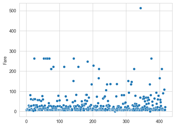
fare = 요금
test_df 에서만 값이 하나가 null 값이다.
중위값으로 채우도록 하자
In [119]:
# scatter plot 으로 확인한 결과 각 값의 이상치가 많으므로 표준 편차가 크기 나온다
# 그러므로 평균값 대신 중위값을 이용하여 na 값을 채우도록 한다.
test_df['Fare'].fillna(test_df['Fare'].median() , inplace = True)
sns.scatterplot(test_df['Fare'])
plt.show()
In [120]:
# 요금의 값이 실수로 되어있는 것을 알수 있다.
# 이를 정수형으로 변환 한다.
print(test_df['Fare'].dtype)
test_df['Fare'] = test_df['Fare'].astype(int)
train_df['Fare'] = train_df['Fare'].astype(int)
float64
In [121]:
# 생존자와 사망자가 낸 요금 의 평군을 비교하여 보자

fare_survived_pivot = \
train_df.loc[:,("Fare","Survived")]\
.pivot_table(columns='Survived', aggfunc = ('std','mean'))\
.loc['Fare']\
.T.reset_index()

train_df['Fare'].plot(kind='hist', figsize=(15,3),bins=100, xlim=(0,50))
plt.show()
plt.figure(figsize=(15,10))
sns.barplot(x = 'Survived' , y= 'mean',data = fare_survived_pivot)
plt.show()

plt.figure(figsize=(15,10))
sns.barplot(x = 'Survived' , y= 'std',data = fare_survived_pivot)
plt.show()


Age = 나이
In [122]:
# Age 는 train,test 둘다 null 값이 많이 존재 한다,
# 이를 해결해보자
# 1 == 세로 개수 2== 가로 개수
fig,( origin_axis  , new_axis) = plt.subplots(1,2,figsize = (20,10))
origin_axis.set_title('Oringinal Age')
new_axis.set_title('New Age')

# avg , std , na 값 개수, 값을 구한다.
avg_age_train_df = train_df['Age'].mean()
std_age_train_df = train_df['Age'].std()
age_na_count_train_df = train_df['Age'].isna().sum()

avg_age_test_df = test_df['Age'].mean()
std_age_test_df = test_df['Age'].std()
age_na_count_test_df = test_df['Age'].isna().sum()

# avg - std ~ avg + std  사이의 임의의 수를 생성한다.
rand_age_for_train = \
np.random.randint(avg_age_train_df - std_age_train_df,
                  avg_age_train_df + std_age_train_df,
                 size = age_na_count_train_df)

rand_age_for_test = \
np.random.randint(avg_age_test_df - std_age_test_df,
                  avg_age_test_df + std_age_test_df,
                 size = age_na_count_test_df)

# na값을 제화한 나머지 값들의 히스토그램을 그린다,
train_df['Age'].dropna().astype('int32').hist(bins = 60  , ax = origin_axis)

# 아까 생성한 표준과 표준편차를 이용한 값을 사용하여 구한 랜덤값 리스트를 이용하여
# na 값을 채운다.
train_df['Age'][np.isnan(train_df['Age'])] = rand_age_for_train
test_df['Age'][np.isnan(test_df['Age'])] = rand_age_for_test

# test,train 전부 나이 값이 float64 로 되어 있으므로 전부 정수형으로 바꾸어 준다
train_df['Age'] = train_df['Age'].astype('int32')
test_df['Age'] = test_df['Age'].astype('int32')

# 결측값을 채운 Age값을 히스토그램으로 그린다.
train_df['Age'].hist(bins = 60 , ax = new_axis)
/var/folders/qg/ktrysd2n07s7yy4yg05vm37h0000gn/T/ipykernel_13577/1812080846.py:33: SettingWithCopyWarning:
A value is trying to be set on a copy of a slice from a DataFrame

See the caveats in the documentation: https://pandas.pydata.org/pandas-docs/stable/user_guide/indexing.html#returning-a-view-versus-a-copy
  train_df['Age'][np.isnan(train_df['Age'])] = rand_age_for_train
/var/folders/qg/ktrysd2n07s7yy4yg05vm37h0000gn/T/ipykernel_13577/1812080846.py:34: SettingWithCopyWarning:
A value is trying to be set on a copy of a slice from a DataFrame

See the caveats in the documentation: https://pandas.pydata.org/pandas-docs/stable/user_guide/indexing.html#returning-a-view-versus-a-copy
  test_df['Age'][np.isnan(test_df['Age'])] = rand_age_for_test
Out[122]:
<Axes: title={'center': 'New Age'}>
In [123]:
# 계속 나이값을 시각화 해보자

# 생존자와 사망자의 나이의 피크값을 알아보자
fig, (axis1,axis2) = plt.subplots(2,1,figsize = (18,10))

sns.kdeplot(x = "Age",
            data = train_df ,
            hue = "Survived",
            shade = True ,
            ax = axis1,
           )
plt.xlim(0, train_df["Age"].max())

# 생존자의 나이에 따른 생존확률

avg_age = train_df[["Age","Survived"]].groupby(["Age"], as_index=False).mean()

sns.barplot(x = "Age" , y = "Survived" , data = avg_age , ax = axis2)
/var/folders/qg/ktrysd2n07s7yy4yg05vm37h0000gn/T/ipykernel_13577/2766721832.py:6: FutureWarning:

`shade` is now deprecated in favor of `fill`; setting `fill=True`.
This will become an error in seaborn v0.14.0; please update your code.

  sns.kdeplot(x = "Age",
Out[123]:
<Axes: xlabel='Age', ylabel='Survived'>
cabin = 선실
cabin의 경우 결측값이 반이상 이기 때문에 아예 제거해 버리겠다..
In [124]:
# cabin
train_df.drop("Cabin", axis = 1 , inplace = True)
test_df.drop("Cabin", axis = 1 , inplace = True)
Family = 같이탄 가족 수
여기서 Family = Parch(부모 자식) + SibSp(같이탄 형제 배우자)
In [125]:
# 가족 컬럼 추가
train_df["Family"] = train_df['Parch'] + train_df['SibSp']
test_df["Family"] = test_df['Parch'] + test_df['SibSp']
# Parch, SibSp 컬럼 제거
train_df.drop(['Parch','SibSp'] ,axis = 1, inplace = True)
test_df.drop(['Parch','SibSp'] ,axis = 1, inplace = True)
#
In [126]:
# 가족수와 생존 확률 비교
avg_family = \
train_df[['Family','Survived']].groupby('Family',as_index=False).mean()
plt.figure(figsize=(10,10))
sns.barplot(x='Family', y = 'Survived',data =avg_family)
Out[126]:
<Axes: xlabel='Family', ylabel='Survived'>
생존확률과 가족 존재 여부는 상관관계가 보이나 가족수가 많을 수록 생존확률이 많아지는 것은 아니다.
그러므로 가족 존재 여부로 바꾼다,
In [127]:
# 가족 존재 여부로 변환
train_df["Family"].loc[train_df["Family"]>0] = 1
test_df["Family"].loc[test_df["Family"]>0] = 1
/var/folders/qg/ktrysd2n07s7yy4yg05vm37h0000gn/T/ipykernel_13577/2680595693.py:2: SettingWithCopyWarning:
A value is trying to be set on a copy of a slice from a DataFrame

See the caveats in the documentation: https://pandas.pydata.org/pandas-docs/stable/user_guide/indexing.html#returning-a-view-versus-a-copy
  train_df["Family"].loc[train_df["Family"]>0] = 1
/var/folders/qg/ktrysd2n07s7yy4yg05vm37h0000gn/T/ipykernel_13577/2680595693.py:3: SettingWithCopyWarning:
A value is trying to be set on a copy of a slice from a DataFrame

See the caveats in the documentation: https://pandas.pydata.org/pandas-docs/stable/user_guide/indexing.html#returning-a-view-versus-a-copy
  test_df["Family"].loc[test_df["Family"]>0] = 1
In [128]:
# 위를 이용한 시각화
fig , (axis1 , axis2) = plt.subplots(1,2,figsize = (10,10))

# 가족 존재 여부와 생존 여부 판단.
avg_family_survived = \
train_df[['Family','Survived']]\
.groupby('Family', as_index=False).mean()

# countplot 과 barplot 사용
sns.countplot(x='Family', data = train_df , ax = axis1)
sns.barplot(x= "Family" ,y= 'Survived', data = train_df , ax = axis2)

# 라벨 설정
axis1.set_xticklabels(['Alone','With Family'])
axis2.set_xticklabels(['Alone','With Family'])

plt.show()

sex = 성
위의 나이 그래프에 따르면 성별외로 나이가 어린 사람의 생존율이 좀 더 높았다
그래서 성을 male , female , child 로 나눈다.
그 후 one-hot incoding 을 사용하여 수치화 해준다.
In [129]:
# 15세 이하의 사람을 어린이로 본다.
# 'sex' column 을 이용하여 person 을 column을 만든다.
# 단일 컬럼에는 map ,apply 을 사용할 수 있지만 , 다중 컬럼일 경우에는 apply에 axis = 1
# 인수를 주고 사용해야 한다.
# apply 에 사용하기 위한 함수 정의
def get_person(person):
    age, sex = person
    return sex if age>15 else 'child'

# apply를 사용하여 person 컴럼 생성
train_df['person'] = train_df[['Age','Sex']].apply(get_person,axis = 1)
test_df['person'] = test_df[['Age','Sex']].apply(get_person,axis = 1)

# sex columns drop
train_df.drop('Sex' ,axis = 1, inplace = True)
test_df.drop('Sex' ,axis = 1, inplace = True)

# 원-핫 인코딩
person_dummies_train = pd.get_dummies(train_df['person'])
person_dummies_test = pd.get_dummies(test_df['person'])
# 컬럼명 변경
person_dummies_train.columns = ['Child', 'Female', 'Male']
person_dummies_test.columns = ['Child', 'Female', 'Male']

# join 은 옆에 부치는 것 concat 은 아래에 부티는 것
train_df = train_df.join(person_dummies_train)
test_df = test_df.join(person_dummies_test)

# subplots 설정
f , (axis1,axis2) = plt.subplots(1,2,figsize = [20,20])

# person 의 카테고리별 count
sns.countplot(x = 'person' , data = train_df ,ax = axis1)

#person 의 카테고리별 생존률
avg_survived_person = \
train_df[['person', 'Survived']].groupby('person',as_index =False).mean()

sns.barplot(x = 'person' ,
            y = 'Survived',
            data = avg_survived_person ,
            ax = axis2,
            order= ['male','female','child'])
plt.show()

# 다쓴 person drop
train_df.drop('person' , axis = 1, inplace = True)
test_df.drop('person' , axis = 1, inplace = True)

# 남성이 제일 많았지만 여성과 아이의 생존 비율이 훨씬 높다.

pclass = 승객 등급
결측값은 없다.
In [130]:
# sns.factorplot('Pclass',data=train_df,kind='count')
# seaborn 0.9.0 부터 바꾸어서 아래와 같이 사용해야 한다고 한다.
# 출처 : https://stackoverflow.com/questions/56077654/trouble-using-factorplot-method-of-seaborn
sns.catplot(x = 'Pclass', y = 'Survived', data = train_df,kind = 'point')
Out[130]:
<seaborn.axisgrid.FacetGrid at 0x28851c220>
1,2,3 등급 밖에 없으므로 이 또한 one-hot-encoding 을 사용한다.
In [131]:
# one-hot-encoding 을 사용하고 컬럼 명을 class1, class2, class3 으로 바꾸어 준다.
class_dummies_train = pd.get_dummies(train_df['Pclass'])
class_dummies_train.columns = ['Class1','Class2','Class2']
class_dummies_test = pd.get_dummies(test_df['Pclass'])
class_dummies_test.columns = ['Class1','Class2','Class2']

# usless Pclass drop
train_df.drop('Pclass' ,axis = 1, inplace = True)
test_df.drop('Pclass' ,axis = 1, inplace = True)

# join dummies to df
train_df = train_df.join(class_dummies_train)
test_df = test_df.join(class_dummies_test)
In [132]:
train_df.info()
print("="*50)
test_df.info()
<class 'pandas.core.frame.DataFrame'>
RangeIndex: 891 entries, 0 to 890
Data columns (total 10 columns):
 #   Column    Non-Null Count  Dtype
---  ------    --------------  -----
 0   Survived  891 non-null    int64
 1   Age       891 non-null    int32
 2   Fare      891 non-null    int64
 3   Family    891 non-null    int64
 4   Child     891 non-null    uint8
 5   Female    891 non-null    uint8
 6   Male      891 non-null    uint8
 7   Class1    891 non-null    uint8
 8   Class2    891 non-null    uint8
 9   Class2    891 non-null    uint8
dtypes: int32(1), int64(3), uint8(6)
memory usage: 29.7 KB
==================================================
<class 'pandas.core.frame.DataFrame'>
RangeIndex: 418 entries, 0 to 417
Data columns (total 10 columns):
 #   Column       Non-Null Count  Dtype
---  ------       --------------  -----
 0   PassengerId  418 non-null    int64
 1   Age          418 non-null    int32
 2   Fare         418 non-null    int64
 3   Family       418 non-null    int64
 4   Child        418 non-null    uint8
 5   Female       418 non-null    uint8
 6   Male         418 non-null    uint8
 7   Class1       418 non-null    uint8
 8   Class2       418 non-null    uint8
 9   Class2       418 non-null    uint8
dtypes: int32(1), int64(3), uint8(6)
memory usage: 14.0 KB
Targert 값과 Feature 값을 분리
In [138]:
# train valid 나누어서 모델 확인
train , valid = train_test_split(train_df , test_size=0.2 , random_state=42)

# Survived drop
X_train = train.drop('Survived' ,axis =1)
X_valid = valid.drop('Survived' ,axis =1)
# only survived
Y_train = train['Survived']
Y_valid = valid['Survived']
# train 과 feature 값을 맞추어 주기 위하여 PassengerId를 제거
X_test = test_df.drop('PassengerId' , axis =1).copy()
Logistic Regression (로지스틱 회귀)
In [139]:
lr_model = LogisticRegression()

lr_model.fit(X_train,Y_train)

Y_pred = lr_model.predict(X_test)

lr_model.score(X_valid,Y_valid)
/opt/homebrew/Caskroom/miniconda/base/lib/python3.10/site-packages/sklearn/linear_model/_logistic.py:458: ConvergenceWarning: lbfgs failed to converge (status=1):
STOP: TOTAL NO. of ITERATIONS REACHED LIMIT.

Increase the number of iterations (max_iter) or scale the data as shown in:
    https://scikit-learn.org/stable/modules/preprocessing.html
Please also refer to the documentation for alternative solver options:
    https://scikit-learn.org/stable/modules/linear_model.html#logistic-regression
  n_iter_i = _check_optimize_result(
Out[139]:
0.7653631284916201In [140]:
svx_model = SVC()

svx_model.fit(X_train , Y_train)

svx_model.score(X_valid, Y_valid)
Out[140]:
0.6536312849162011In [141]:
rf_model = RandomForestClassifier(n_estimators=100)

rf_model.fit(X_train,Y_train)

rf_model.score(X_valid,Y_valid)
Out[141]:
0.7932960893854749최종적으로 Random forest 가 가장 뛰어난 성능을 보이므로 해당 모델을 사용하여 결과를 제출한다.
In [151]:
X_train = train_df.drop('Survived' ,axis =1)
# only survived
Y_train = train_df['Survived']
In [153]:
rf_model = RandomForestClassifier(n_estimators=100)

rf_model.fit(X_train,Y_train)

Y_pred = lr_model.predict(X_test)
In [154]:
# 로지스틱 회귀 모델에서 각 Feature별 상관 계수를 가지고 온다.
coeff_df = pd.DataFrame(train_df.columns.delete(0))
coeff_df.columns = ['Features']
coeff_df["Coefficient Estimate"] = pd.Series(lr_model.coef_[0])


coeff_df
Out[154]:
FeaturesCoefficient Estimate012345678
| Age | -0.019551 |
| Fare | 0.001398 |
| Family | -0.232565 |
| Child | 0.519034 |
| Female | 1.420083 |
| Male | -1.465784 |
| Class1 | 1.210193 |
| Class2 | 0.218053 |
| Class2 | -0.954913 |
요금과 나이는 거의 상관이 없다고 나왔다.
In [155]:
submission = pd.DataFrame({
        "PassengerId": test_df["PassengerId"],
        "Survived": Y_pred
    })
submission.to_csv('titanic.csv', index=False)